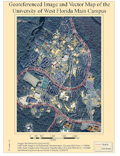
Week 6 - Georeferencing Lab

This was an interesting lab.  I have some experience selecting relative control points so that aided my choices in points. 

Equilateral Triangles

One thing I remembered was thinking about a term called "strength of figure".  Mathematically, the most stable triangle is the equilateral triangle.  Using this thought, I tried to choose my points so that they created a network of triangles that came as close as possible to equilateral triangles.    Just for grins and giggles, I also selected some at random and the RMS error almost doubled. 

Deleting Points

I constantly looked at the RMS errors of individual points and deleted ones that started to get quite large.  I think that I collected them in the wrong order (known to unknown) and that caused some HUGE errors.  So judiciously using the delete key was quite helpful.

Week 5: Data Input and Editing

So the elements that are in this map are

1. County boundaries
2. Cities and towns
3. Public Land
4. Roads
5. Hydrography
6. Land Cover
7. Wetlands

I learned a ton on this lab.  This took soooooo much time but I learned so much.  Thanks to Sean's tip form the Discussion post about the data..  That was wonderful!  The tip was"Open the attribute table for the layer and see if their is a field that describes each row of data....., right click on the layer and selected symbology, then on the left selected show categories. At that point there is probably only 1 category showing that says something like and has a check next to it. Uncheck the check and click the button at the bottom that says Add values or add all values. But before you do that change the Value Field to the field in the attribute table that held the description."  There was so much more data than I knew was there until that point.  Once I understood this, the rest of the lab came together nicely.

Thank goodness the USGS site with their Explorer tool worked.   That is where I downloaded most of the information.  The Florida site had it too but for some reason the download hung up every single time.

The main goal was to import 4 adjacent DOQQ, (the center piece here), and then add an adjacent Digital Elevation Model DEM and Digital Raster Graphic (DRG).  The legend was intentionally left out since the three primary elements were clearly and unambiguously labled.  Per the Thematic Cartography and Geovisualization text, "symbols that are self explanatory ... are normally omitted."

Notice the map collar, is this

Haiti Road Maps

I am a big, big fan of maps.  The advantage of this map is that it is very useful for planning purposes.  The primary drawback to this and many other maps is that the veracity of the source is generally not verifiable.  In this case however, I was able to confirm that some of the "probably closed" roads were in fact, impassable.  How could I do that?  It turns out that  latest update to google imagery was also about that same time.  And the resolution of the imagery was good enough to show that a collapsed building had completely obstructed the road.

Week 4 - Projection Type Comparison

The objective of this lab was to depict the variability of acreage calculations when implementing different geographic projections. This was a very time consuming lab albeit rewarding.

The lab demonstrated how to make changes to datasets in ArcGIS. The three map projections were generated using the ArcGIS ArcToolbox, Projections and Transformations toolset, specifically the Project Tool to create new datasets from the original Albers projection.  Microsoft Excel was used to create the Legend.  I appreciated how products from other vendors (i.e. Microsoft) could be added to enhance the value of the GIS product.